Create an Interactive Game in Microsoft Excel

In this activity you will create an interactive educational game. There will be 9 questions and if they are answered correctly it will reveal a picture underneath.
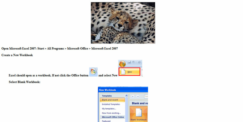
1.The picture we will use for this activity is above.
2.Right click or (drag on a Mac) and Save it to your picture file
3.Rename as lepard.
Insert a Background Picture....
1. First open Excel and go to the Page Layout tab
2. Second click Background to open the Sheet Background dialog box.
3. Next Navigate to the folder that contains the picture you saved above.
4. Finally Click Insert on the Sheet Background dialog box to place the picture on the page.
See below for details.....
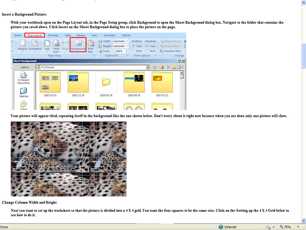
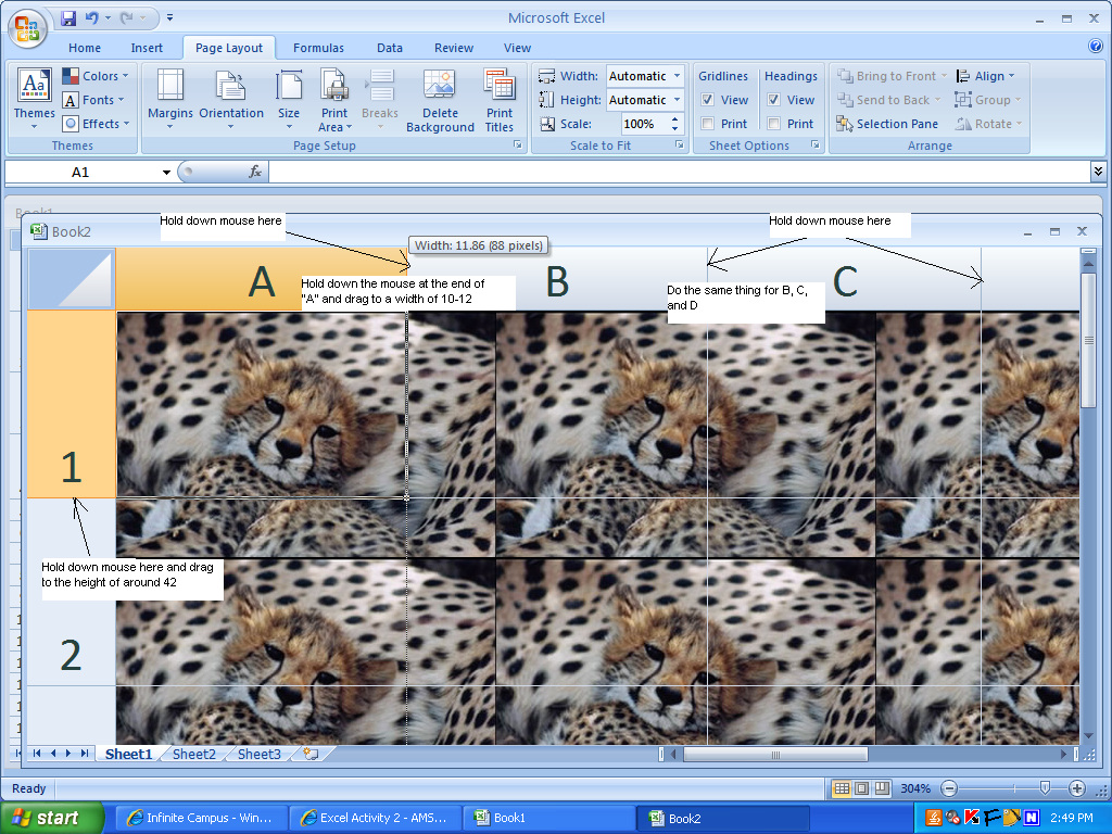
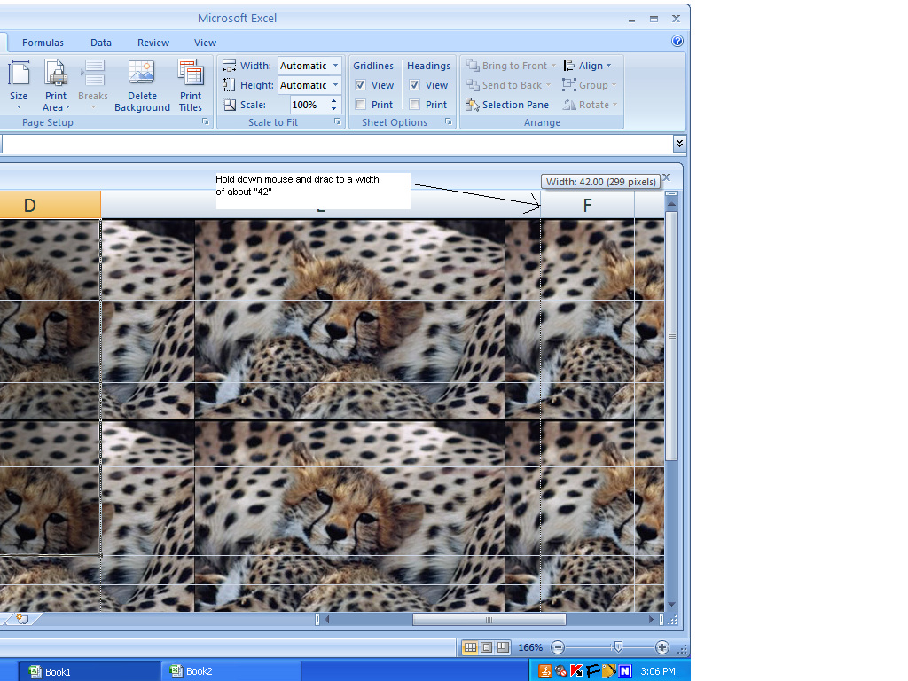
Adjust the picture to a 4x4 grid.....see example below.
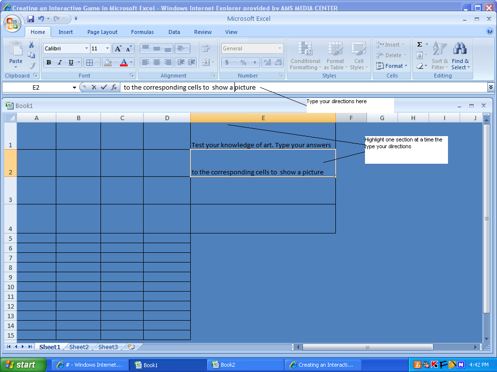
Next you will need to set up the cells that will contain the instructions for your game see example below.
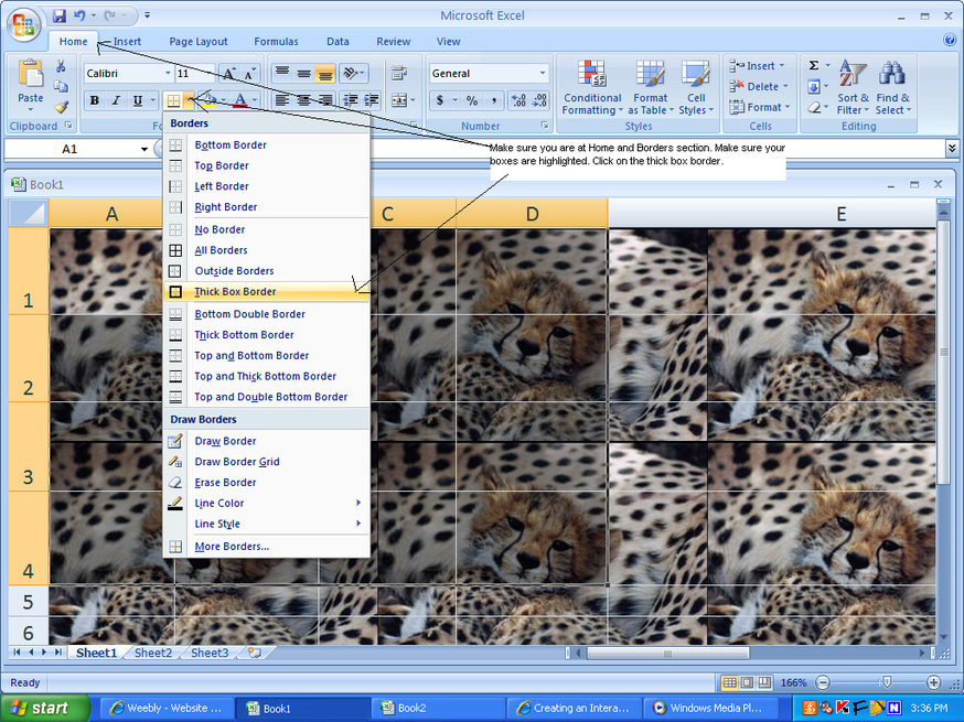
Add borders to your sections A-D and 1-4....
make sure you highlight each square first then
Click on "thick border tab and all border tab"
See example below....
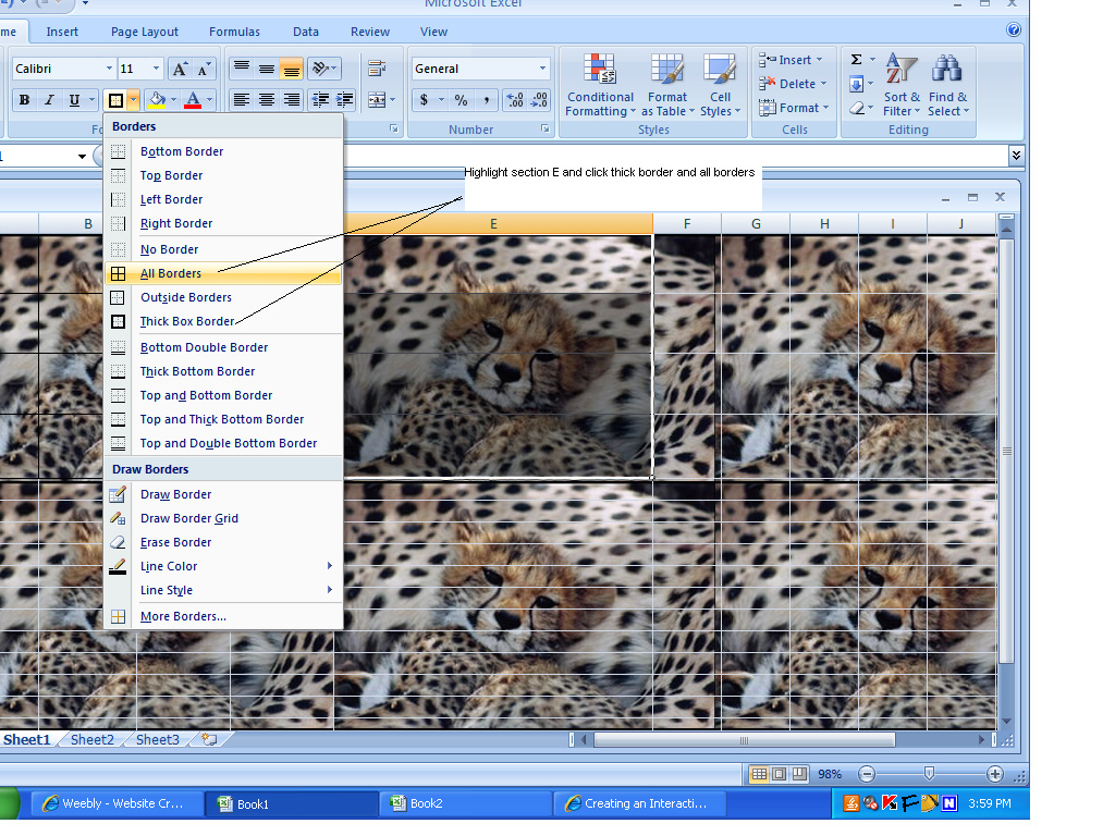
Add borders for your E section highlight then click on "thick border tab and all border tab" see example below.
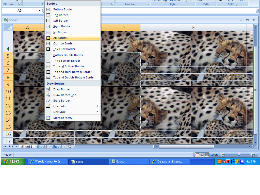
Now add borders for your questions....Highlight 5-15 and A-D sections and click on "thick border tab and all border tab" see example below.
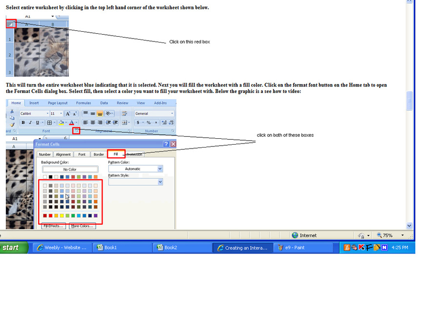
Add fill to the picture...see example below.
Now add the text to your game....See the directions below.
Add your questions...See below example
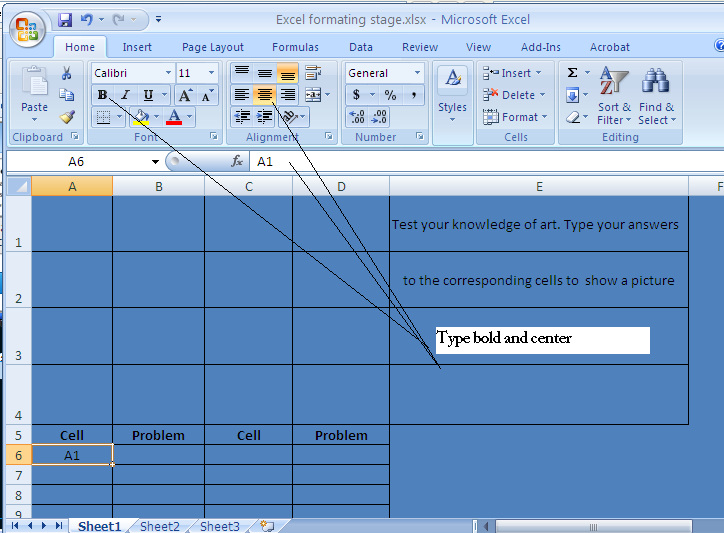
Type all of the cell letters and numbers and your problem questions...
Now add Conditional Formatting to the Picture Squares.
1.First Click in Cell A1 and with the Home tab selected (the picture square)
2.Then click Conditional Formatting
3.Next click Highlight Cell Rules
4.Finally click Equal To
5.Type your answer in the box and click custom format
See below for directions...
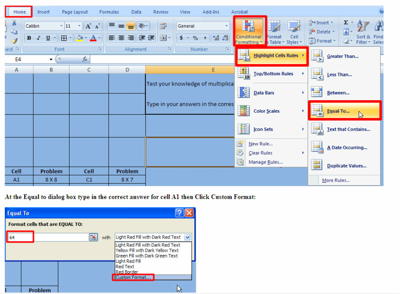
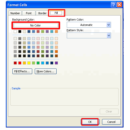
1.At the Format Cells dialog box select the Fill tab and select No Color. Then click OK to apply the conditional formatting to the cell A1.
2.Continue adding conditional formatting to the remainder 15 of the picture cells.
Now we are going to Lock the Worksheet and Unlock Cells.
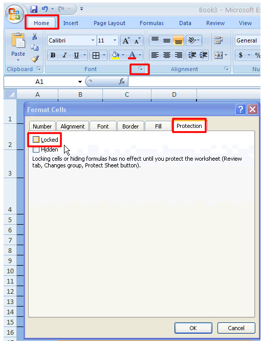
By default all cells are locked so you need to select the cells that contain your picture and unlock them by clicking the Locked box to unlock it. 1.Select the picture cells and with the Home tab selected select the arrow at the bottom corner of the font section.
2.Then click on the Protection tab on the Format Cells dialog box.
3.Click in the Locked section to remove the check.
4.Click OK to apply this formatting.
See directions below.....
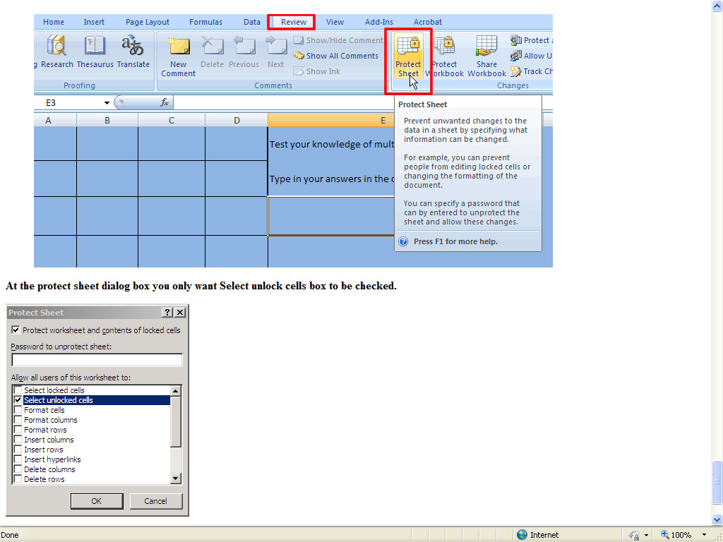
Once you have unlocked the picture cells you will need to protect the worksheet so no one can edit any of the data you have entered. With the Review